Hierarchical Clustering with Python Part 6: Cluster Distances

Don't worry. It's all intuition. There's no math in this one.

May 12, 2026

Are you new to this tutorial series? Check out Part 1 here.

You learned in Part 3 of this tutorial series how the agglomerative hierarchical clustering algorithm calculates the distance between two data points (i.e., rows) in a dataset.

This tutorial will cover the various methods the AgglomerativeClustering class in scikit-learn offers for calculating distances between clusters.

As covered in Part 2 of this tutorial series, the algorithm needs both types of distances to mine the cluster hierarchy (i.e., taxonomy) from a dataset.

These methods for calculating distances between clusters are called linkages. The AgglomerativeClustering class supports four different linkages.

#1 - Single Link

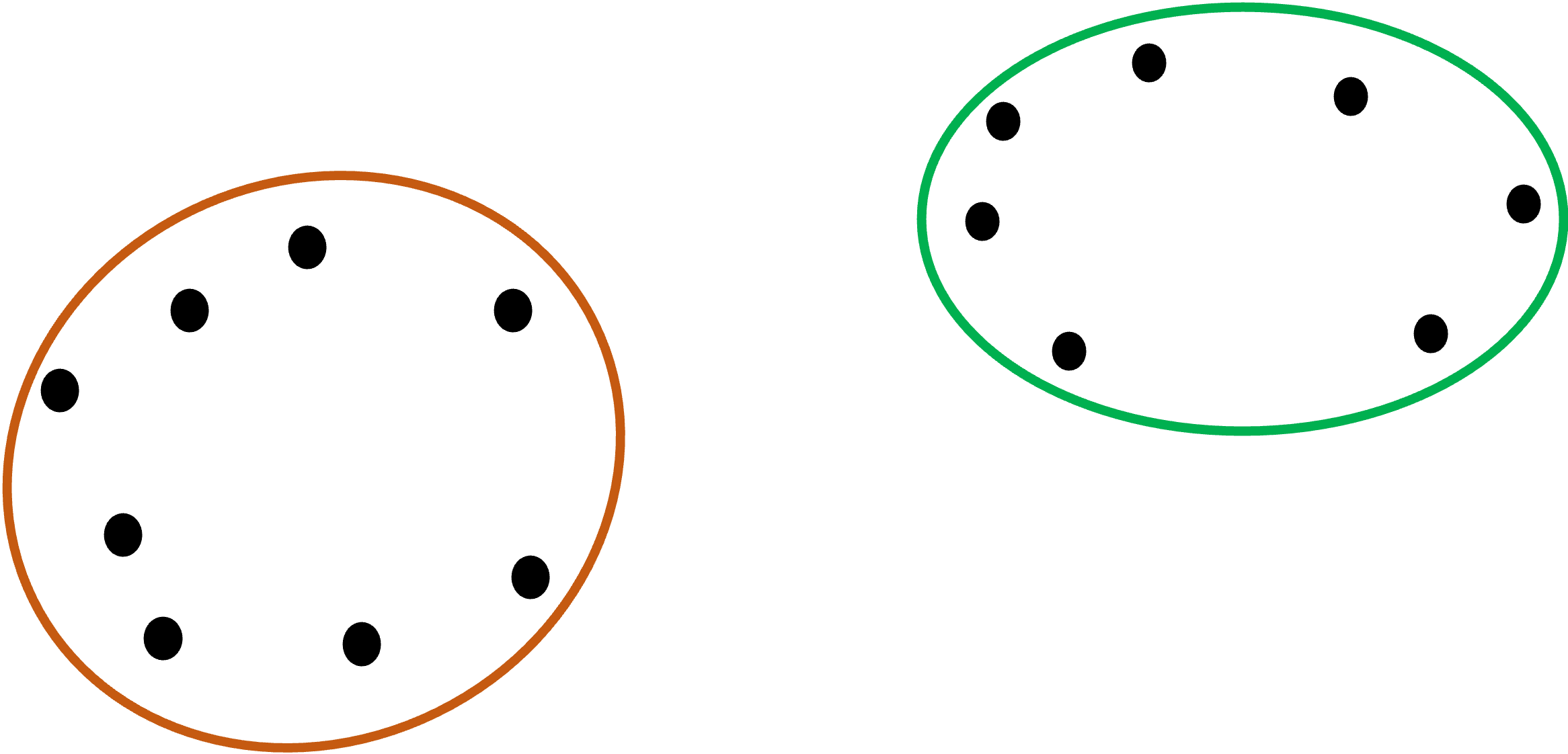
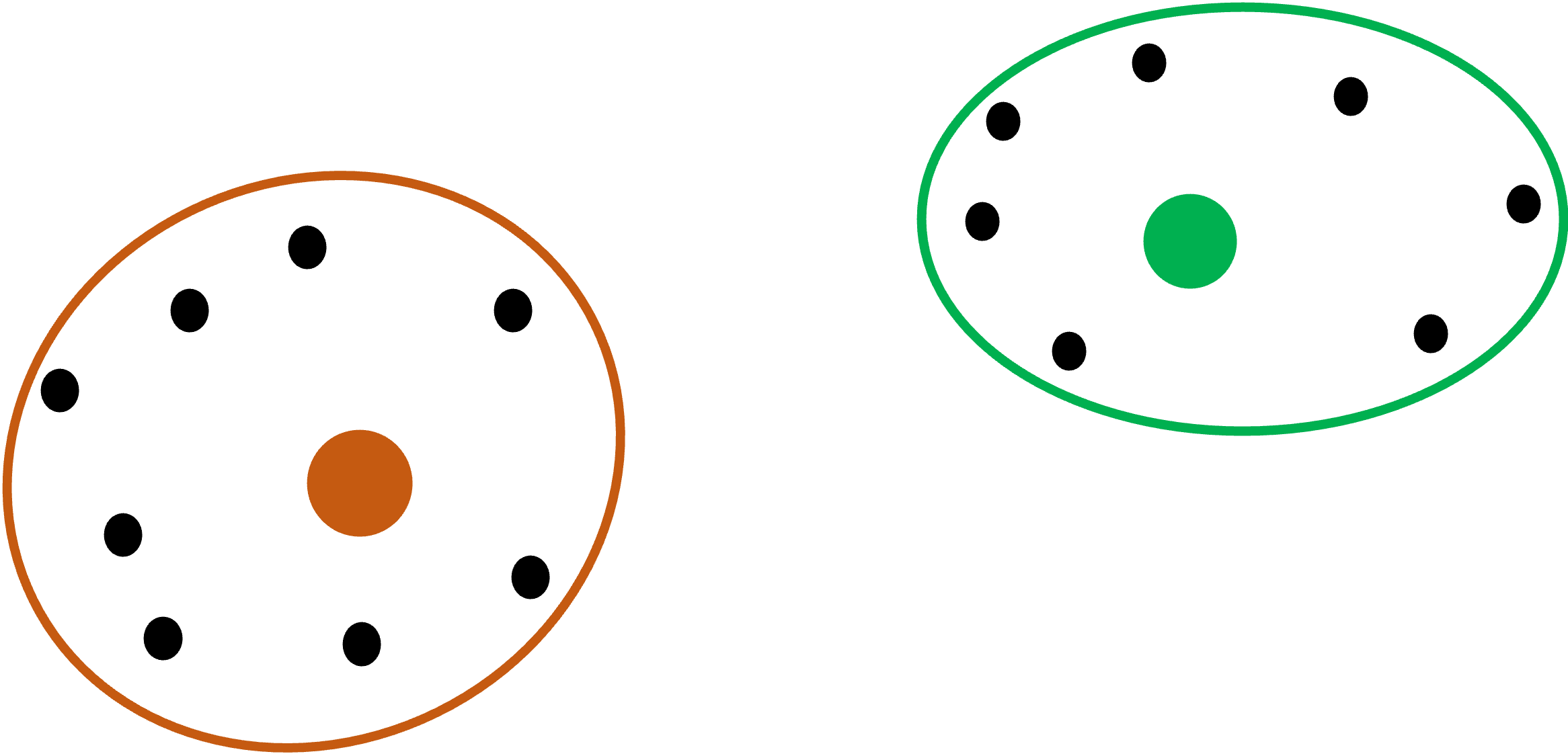
Understanding each linkage type is quite intuitive when you use a graphical representation. For this tutorial, assume we have the following two clusters:

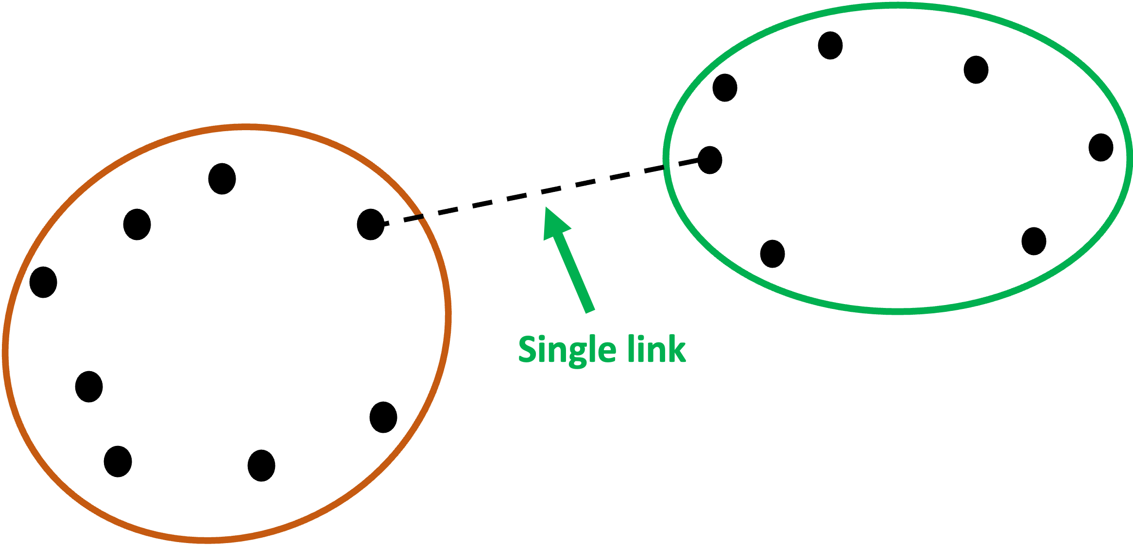
The first linkage is known as single link.

Single link calculates the distances between all the points in each of the clusters and then chooses the smallest of these distances to represent how similar (i.e., close together) the clusters are.

Graphically, single link would use the following two points for the distance between the clusters because it is the minimum:

Here's how to use single link with the AgglomerativeClustering class:

from sklearn.cluster import AgglomerativeClustering

# Use single link for cluster distances
agg_clustering = AgglomerativeClustering(linkage = 'single')

NOTE - This code is the same whether you’re using Python in Excel, VS Code, or Jupyter Notebook.

If you’re new to Python, my Python in Excel Accelerator online course will teach you the fundamentals you need for analytics in a weekend.

#2 - Complete Link

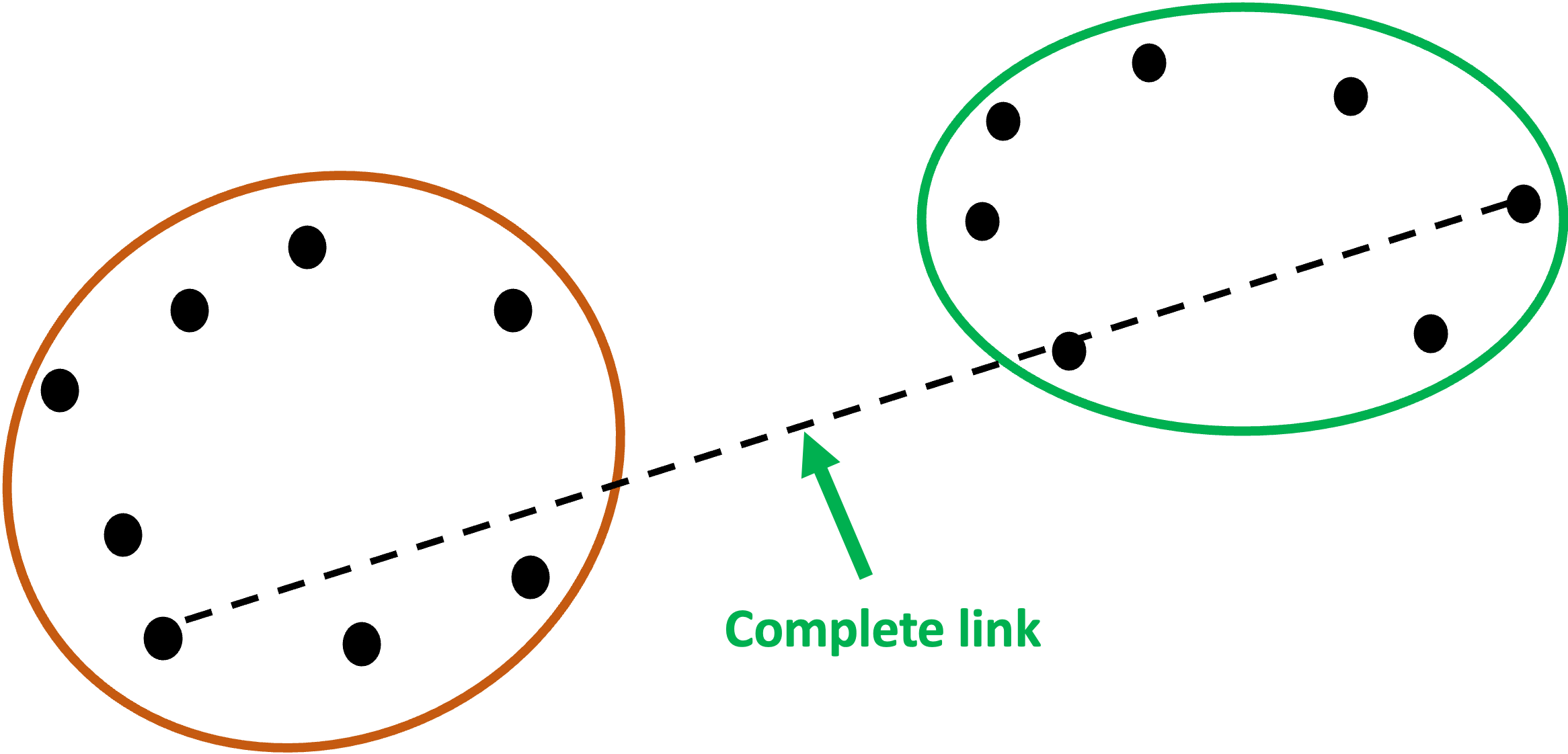
If there’s a linkage that uses the minimum distance between two points in each cluster, it stands to reason that there would be a linkage that uses the maximum distance.

This is known as complete link.

I know.

Why couldn’t they just call them min and max? 🤷‍♂️

Here’s complete link shown graphically:

And in code:

from sklearn.cluster import AgglomerativeClustering

# Use complete link for cluster distances
agg_clustering = AgglomerativeClustering(linkage = 'complete')

#3 - Average Link

The next linkage is the average link. As you might have guessed, this linkage uses the average distance between all data points in two clusters.

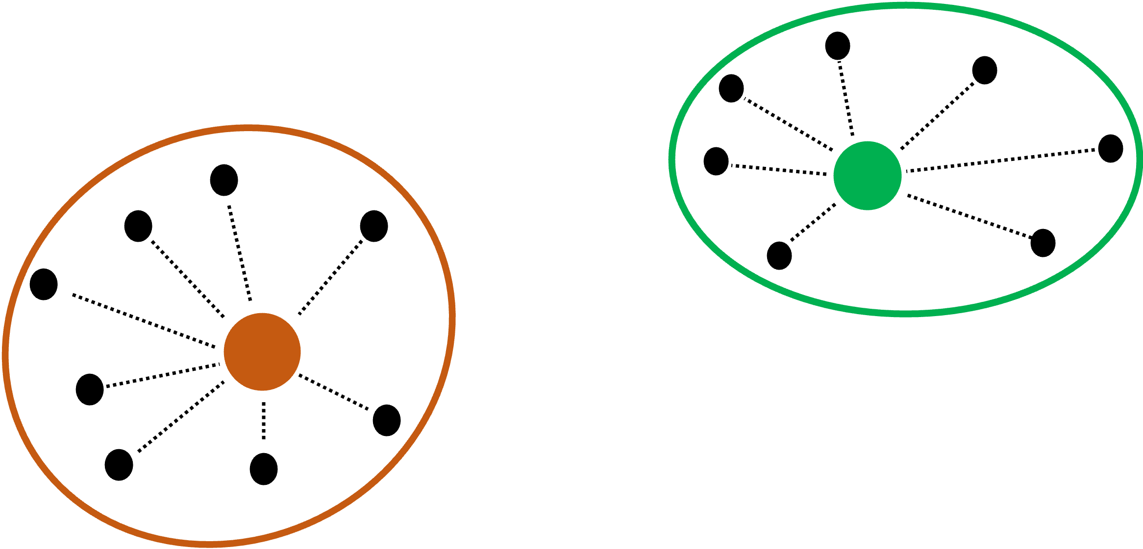
To keep the graphic from being overwhelming, I’ve only included the distance lines for two data points from the orange cluster:

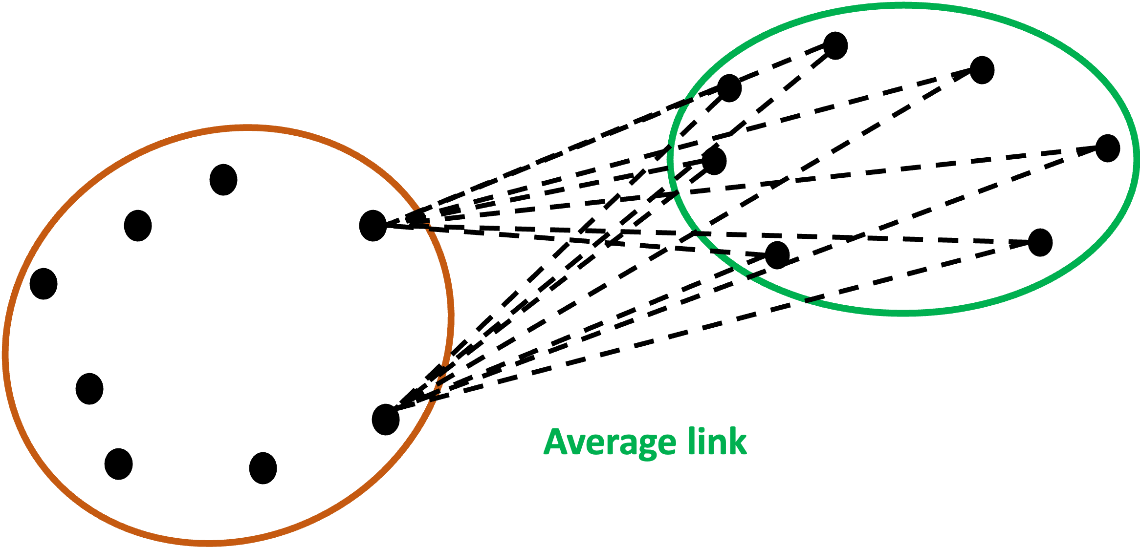
Imagine all the distance lines from every data point in the orange cluster to every data point in the green cluster.

The similarity of the clusters is the average of all those distance lines - a smaller average indicates more similar clusters.

Here’s the code to specify using average link:

from sklearn.cluster import AgglomerativeClustering

# Use Ward's method for cluster distances
agg_clustering = AgglomerativeClustering(linkage = 'average')

#4 - Ward Linkage

The last linkage is the AgglomerativeClustering default: the Ward linkage. The Ward linkage (or Ward’s method) is more involved than the previous linkages.

If you’re familiar with the k-means clustering algorithm (e.g., from my Cluster Analysis with Python online course), then Ward linkage will be familiar to you.

The ward linkage uses prototypes. Think of prototypes as being data points that the algorithm “makes up” to be the center of each cluster.

The most common type of prototype is the centroid, which is the average of all data points in the cluster.

Graphically, the orange and green dots are the centroids of the two clusters in our running example:

The ward linkage first evaluates each cluster by finding all the distances (i.e., the dotted lines) between the data points in a cluster and their centroid:

Consider the orange cluster above. There are eight data points in the cluster and eight distances between each data point and the centroid.

The ward linkage takes each one of these distance values and squares them (i.e., the distance multiplied by itself). It then sums all these squared distances.

It then repeats this process for the green cluster.

Lastly, it then adds the sum of the squared distances for the orange cluster to the sum of the squared distances for the green cluster.

Think of this last calculation (i.e., adding the two sums together) as being the baseline.

The ward linkage then combines the two clusters and calculates a new centroid (represented in blue):

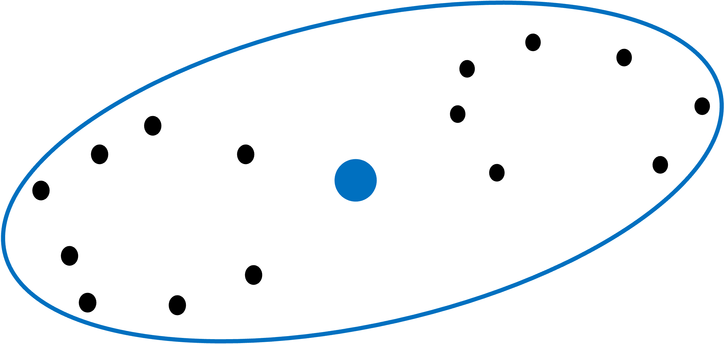
The ward linkage then sums up all the squared distances for the new, larger cluster:

Think of the sum of the squared distances for the new, larger cluster as being the new hotness.

Ward linkage calculates the difference between the baseline and the new hotness, treating it as a penalty for combining clusters. Ward linkage looks to make this penalty as small as possible when considering which clusters to combine.

By minimizing the penalty, ward linkage prioritizes combining the most similar clusters.

Even though Ward’s method is the default, here’s the code for reference:

from sklearn.cluster import AgglomerativeClustering

# Use Ward's method for cluster distances
agg_clustering = AgglomerativeClustering(linkage = 'ward')

Which Linkage to Use?

It shouldn’t come as a surprise that using different linkages can produce different clusterings.

So, you may be asking yourself, “Which linkage should I use?”

When it comes to cluster analysis, I’m a big fan of experimenting to see what works best. For example, using different linkages and seeing which produces the most useful clusters.

That being said, here are some rules of thumb:

Single link is good at handling non-spherical cluster shapes, but is sensitive to outliers.
Complete link is less susceptible to outliers, but can break large clusters, and it tends to produce spherical clusters.
Think of average link as being a compromise between the single and complete linkages.
Think of Ward’s method as being a bit of an improvement over average link.

That’s it for this tutorial.

My next newsletter will be the last in this series. The topic is using ML predictive models to help interpret clusters.

Stay healthy and happy data sleuthing!