Boosted Decision Trees Part 3: Python Code

It's time for you to build the models.

Jul 17, 2026

Are you new to this tutorial series? Check out Part 1 here.

When you use the AdaBoost algorithm in Python, it can seem magical because so much is happening behind the scenes (what I refer to as automagically).

In the past two tutorials, you’ve built an intuitive understanding of what AdaBoost does for you automagically.

In this week's tutorial, you will learn how the AdaBoost algorithm builds an ensemble of weak learners (i.e., decision stumps). You’re going to see how it works step by step using Python code.

And with this foundation, you will be ready for the final two parts of this tutorial series:

How AdaBoost combines weak learners to make predictions.
How to use AdaBoost with the scikit-learn library.

BTW - If you’re new to decision tree machine learning, be sure to check out my recorded live crash course, which includes a PDF of all the slides, data, and code.

Loading the Data

If you would like to follow along with today's tutorial (highly recommended), download the Adult.xlsx file from the newsletter's GitHub repository.

Here's the code for loading this tutorial's dataset using Python in Excel:

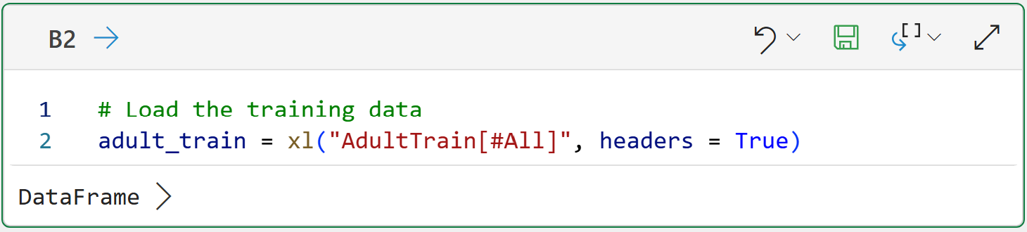
BTW - I will be using Python in Excel for this tutorial series, but 99+% of the code is the same whether you’re using Excel, Jupyter Notebook, or VS Code.

And here’s the code for your Excel workbook:

# Load the training data
adult_train = xl("AdultTrain[#All]", headers = True)

Calling the info() method on adult_train provides you with a lot of info about the dataset:

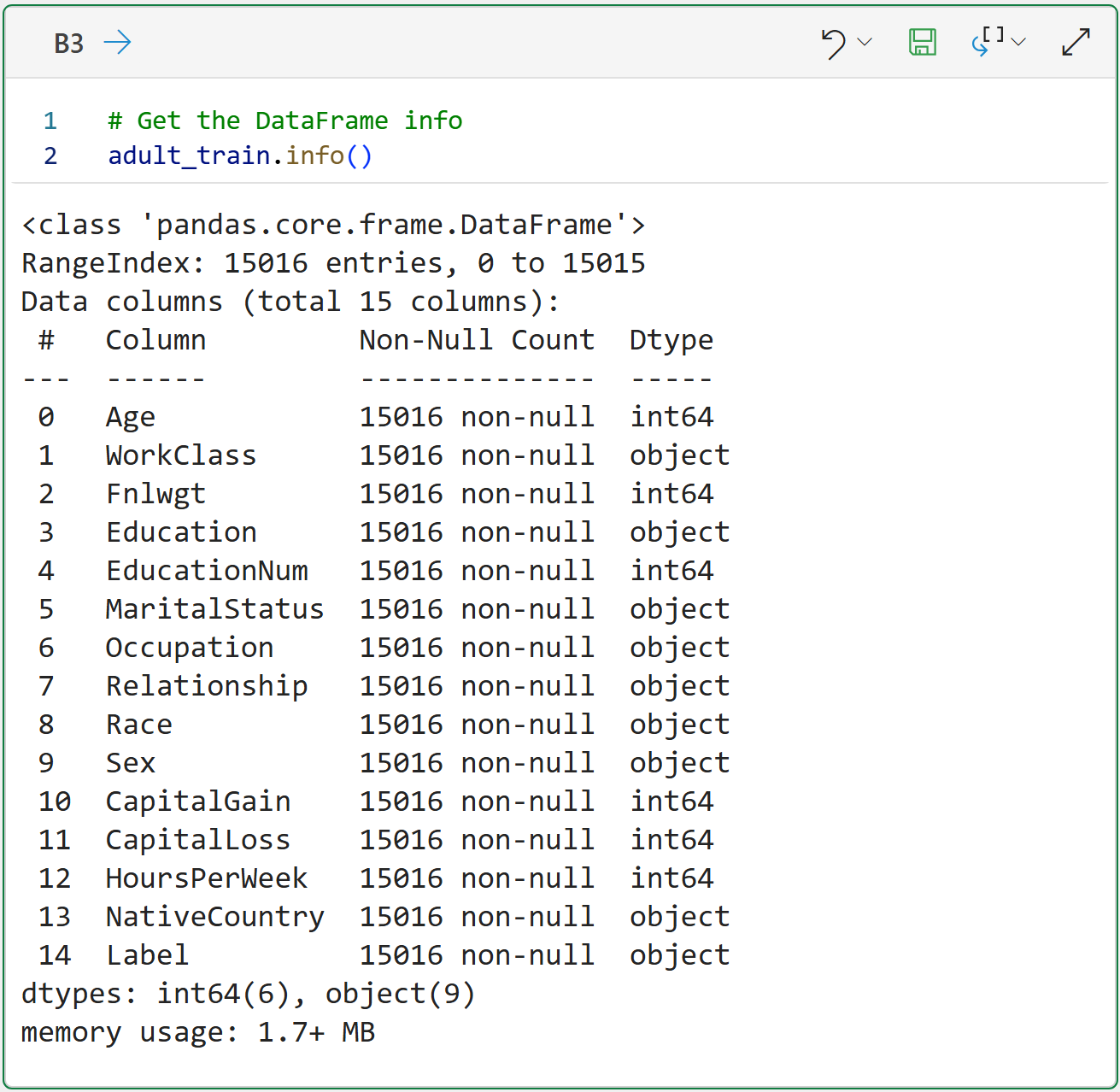
# Get the DataFrame info
adult_train.info()

If you’re interested, you can learn more about this dataset from the UCI Machine Learning Repository.

For our purposes, this dataset embodies a predictive modeling task where:

Label represents the income of a US resident of either more than $50,000 per year (i.e., Label value of >50K) or less (i.e., Label value of <=50K).
The rest of the features are characteristics of US residents (e.g., Age, Education, HoursPerWeek, etc.)

The AdaBoost algorithm will build an ensemble of weak learners (i.e., decision stumps) to accurately predict the Label based on the available features.

For this tutorial, I will be using a subset of the available features to keep things simple:

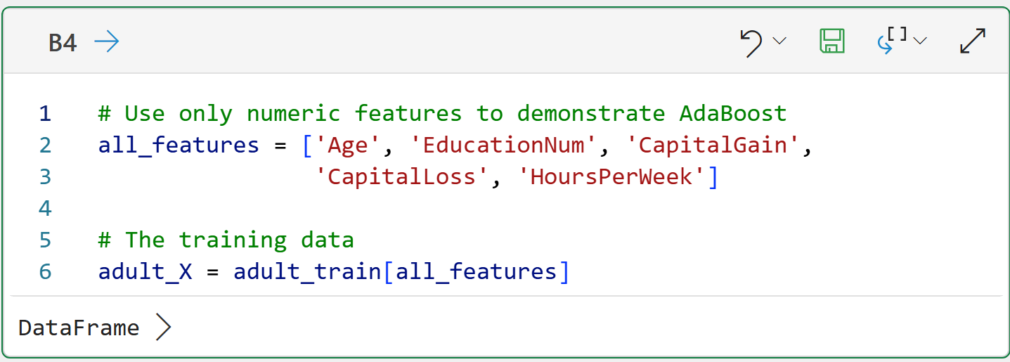
# Use only numeric features to demonstrate AdaBoost
all_features = ['Age', 'EducationNum', 'CapitalGain',
                'CapitalLoss', 'HoursPerWeek']

# The training data
adult_X = adult_train[all_features]

Also, the Label feature consists of string values, so encoding them to be numeric is a good idea:

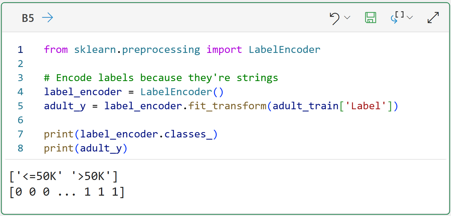
from sklearn.preprocessing import LabelEncoder

# Encode labels because they're strings
label_encoder = LabelEncoder()
adult_y = label_encoder.fit_transform(adult_train['Label'])

print(label_encoder.classes_)
print(adult_y)

The classic AdaBoost algorithm takes only one input from you - the number of weak learners in the ensemble. This is often referred to as the number of boosting rounds, since each round produces a weak learner.

For this tutorial, we’ll use three boosting rounds to demonstrate how AdaBoost works step by step.

However, the number of boosting rounds may not be optimal for the tutorial’s dataset. I arbitrarily selected three for this tutorial.

Boosting Round #1

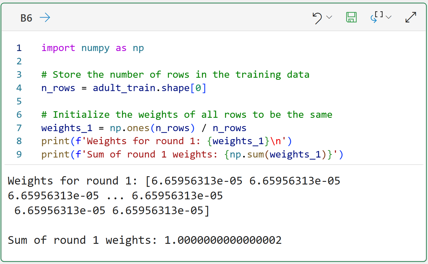
As covered in Part 2 of this tutorial series, the first step in AdaBoost is to create the initial weights for each row in the training dataset, where each weight is the same for Round #1:

import numpy as np

# Store the number of rows in the training data
n_rows = adult_train.shape[0]

# Initialize the weights of all rows to be the same
weights_1 = np.ones(n_rows) / n_rows
print(f'Weights for round 1: {weights_1}\n')
print(f'Sum of round 1 weights: {np.sum(weights_1)}')

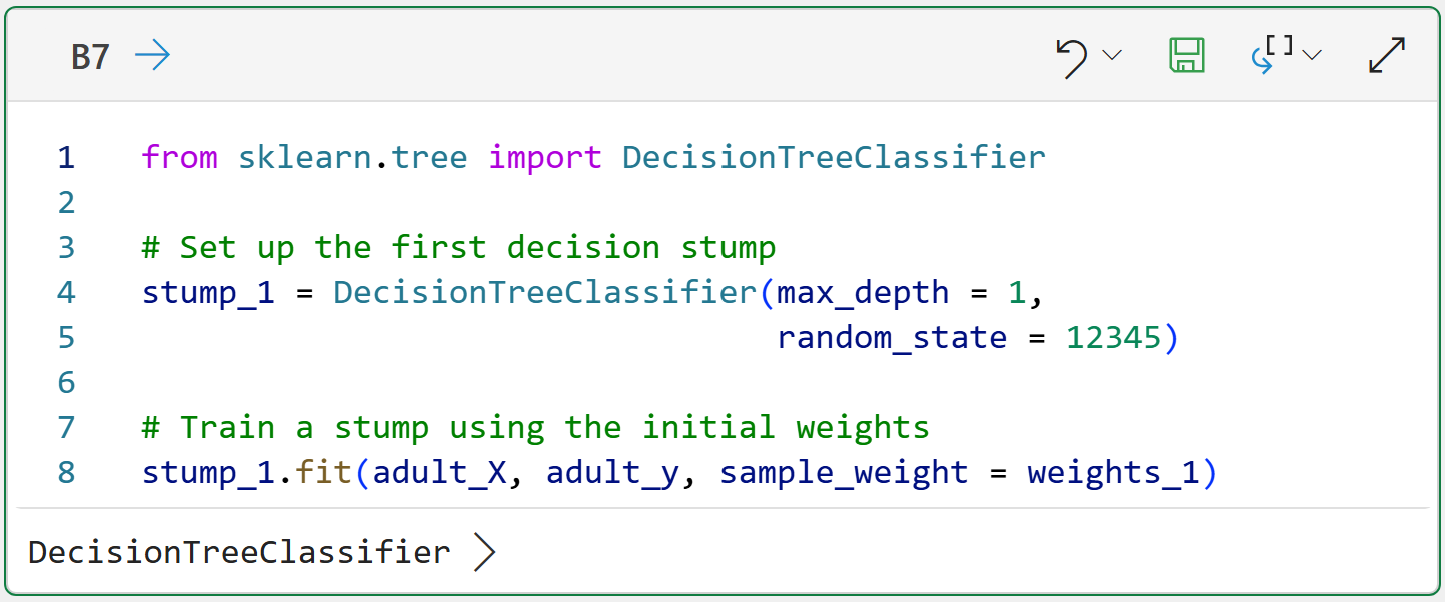
With the initial weights calculated, the next step is to train a weak learner. In the case of the classic AdaBoost algorithm, the weak learner is a decision stump:

from sklearn.tree import DecisionTreeClassifier

# Set up the first decision stump
stump_1 = DecisionTreeClassifier(max_depth = 1, 
                                 random_state = 12345)

# Train a stump using the initial weights
stump_1.fit(adult_X, adult_y, sample_weight = weights_1)

The code above creates an instance of the DecisionTreeClassifier class from the scikit-learn library. By setting the max_depth hyperparameter to 1, the trained model will be a decision stump.

The magic of AdaBoost happens on line 8 of the above code, where the sample_weight parameter is used in the call to fit().

In this case, since all weights are the same, they don’t have much impact on the learning process for the decision stump. As you will see later, weights have a significant effect.

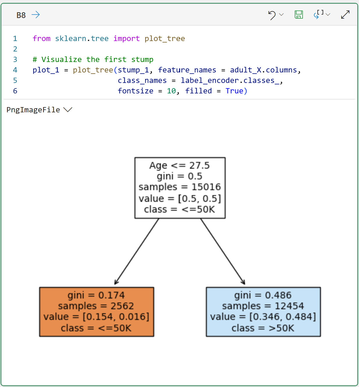
The following code visualizes the first weak learner in the ensemble:

from sklearn.tree import plot_tree

# Visualize the first stump
plot_1 = plot_tree(stump_1, feature_names = adult_X.columns, 
                   class_names = label_encoder.classes_,
                   fontsize = 10, filled = True)

As shown above, the first weak learner in the ensemble has selected the rule Age <= 27.5 for making its predictions. Not surprisingly, this isn’t very good in terms of its predictive performance (e.g., accuracy).

For example, for dataset rows where Age > 27.5, the above decision stump model is only slightly better than 50/50 in making predictions (i.e., the gini is close to 0.5).

Not to worry, outcomes like this are by design with the AdaBoost algorithm.

Boosting Round #2

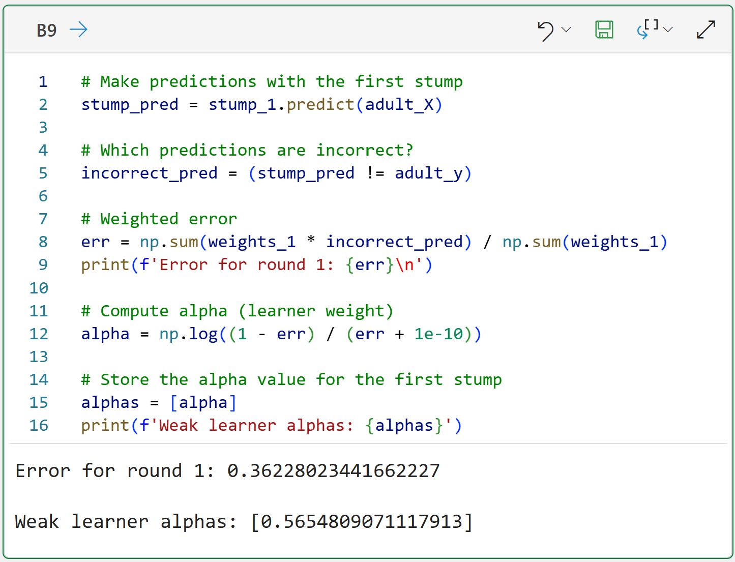
With the first weak learner in place, the AdaBoost algorithm uses the predictions from the first decision stump to weight the data for the second boosting round.

The intuition here is that the weighting will make the next weak learner focus on the predictions the previous weak learner got wrong:

# Make predictions with the first stump
stump_pred = stump_1.predict(adult_X)

# Which predictions are incorrect?
incorrect_pred = (stump_pred != adult_y)

# Weighted error
err = np.sum(weights_1 * incorrect_pred) / np.sum(weights_1)
print(f'Error for round 1: {err}\n')

# Compute alpha (learner weight)
alpha = np.log((1 - err) / (err + 1e-10))

# Store the alpha value for the first stump
alphas = [alpha]
print(f'Weak learner alphas: {alphas}')

As covered in Part 2, think of the alpha as the importance score for the weak learner. Given that the first weak learner’s error was less than 0.5 (i.e., 0.36228), it received a positive alpha score of 0.565481.

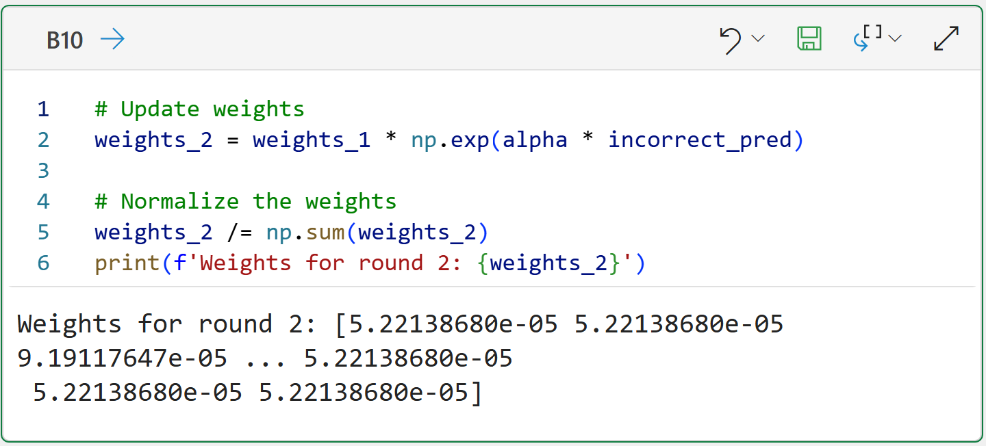
With the erroneous predictions identified and the first weak learner’s alpha score calculated, AdaBoost then updates the dataset weights for the next weak learner to focus on better predicting the errors:

# Update weights
weights_2 = weights_1 * np.exp(alpha * incorrect_pred)

# Normalize the weights
weights_2 /= np.sum(weights_2)
print(f'Weights for round 2: {weights_2}')

In the output above, take a look at the Round #2 weights and compare them to the Round #1 weights. In particular, compare the first three Round #2 weights to the first three Round #1 weights:

Round #2 weights:

5.22138680e-05
5.22138680e-05
9.19117647e-05

Round #1 weights:

6.65956313e-05
6.65956313e-05
6.65956313e-05

The Round #2 values illustrate how the weights are adjusted to give higher weights to errors (e.g., the third row of the dataset as represented by the third bullet).

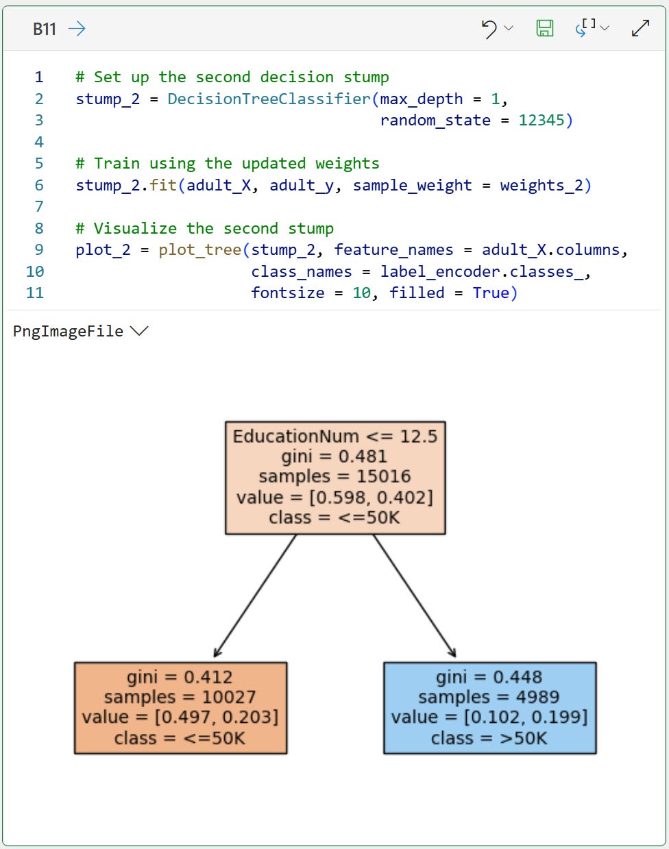
With the updated weights calculated, a second weak learner is added to the ensemble:

# Set up the second decision stump
stump_2 = DecisionTreeClassifier(max_depth = 1, 
                                 random_state = 12345)

# Train using the updated weights
stump_2.fit(adult_X, adult_y, sample_weight = weights_2)

# Visualize the second stump
plot_2 = plot_tree(stump_2, feature_names = adult_X.columns,
                   class_names = label_encoder.classes_, 
                   fontsize = 10, filled = True)

The above decision stump demonstrates the power of the AdaBoost algorithm.

Because of the updated weights, the second decision stump has focused on the EducationNum feature as the best way to address the first stump's errors.

However, AdaBoost isn’t done yet because we’re assuming three boosting rounds.

Boosting Round #3

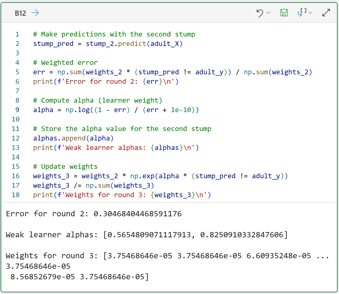
The same process is just repeated, starting with finding the errors for the second weak learner:

# Make predictions with the second stump
stump_pred = stump_2.predict(adult_X)

# Weighted error
err = np.sum(weights_2 * (stump_pred != adult_y)) / np.sum(weights_2)
print(f'Error for round 2: {err}\n')

# Compute alpha (learner weight)
alpha = np.log((1 - err) / (err + 1e-10))

# Store the alpha value for the second stump
alphas.append(alpha)
print(f'Weak learner alphas: {alphas}\n')

# Update weights
weights_3 = weights_2 * np.exp(alpha * (stump_pred != adult_y))
weights_3 /= np.sum(weights_3)
print(f'Weights for round 3: {weights_3}\n')

Check out the error and alpha for the second weak learner in the output above.

Because the second weak learner has a lower error than the first, it has a higher alpha score of 0.825091 compared to 0.565481.

As you will learn in the next tutorial, the second weak learner will be considered more important than the first weak learner in making predictions.

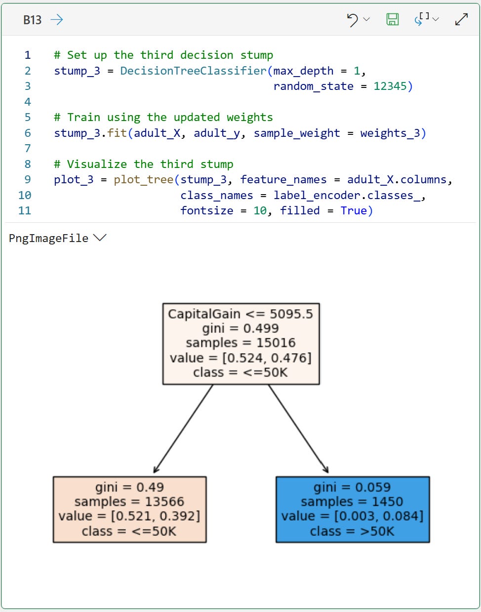
Again, with the weights updated, the final weak learner can be added to the ensemble:

# Set up the third decision stump
stump_3 = DecisionTreeClassifier(max_depth = 1, 
                                 random_state = 12345)

# Train using the updated weights
stump_3.fit(adult_X, adult_y, sample_weight = weights_3)

# Visualize the third stump
plot_3 = plot_tree(stump_3, feature_names = adult_X.columns,
                   class_names = label_encoder.classes_, 
                   fontsize = 10, filled = True)

Notice how the third decision stump has chosen the CapitalGain feature to address the errors of the second decision stump?

This is core to using machine learning ensembles: to achieve better predictive performance, the ensemble models should be significantly different from each other.

As you can see, the AdaBoost algorithm’s use of weights and decision stumps ensures the models are as different from each other as possible.

And the alpha for the final weak learner:

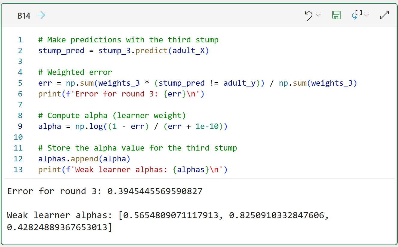
# Make predictions with the third stump
stump_pred = stump_3.predict(adult_X)

# Weighted error
err = np.sum(weights_3 * (stump_pred != adult_y)) / np.sum(weights_3)
print(f'Error for round 3: {err}\n')

# Compute alpha (learner weight)
alpha = np.log((1 - err) / (err + 1e-10))

# Store the alpha value for the third stump
alphas.append(alpha)
print(f'Weak learner alphas: {alphas}\n')

The output above for the third weak learner illustrates an important concept in boosted decision trees.

Inevitably, there are diminishing returns for adding more models to the ensemble. In the worst case, adding too many models can reduce the ensemble's predictive performance.

In the case of AdaBoost, tuning the ensemble model involves determining the optimal number of weak learners for a given dataset.

👉 Ready to learn more? Check out Part 4 here.

That’s it for this tutorial.

The next tutorial in this series will cover how the AdaBoost algorithm combines weak learners to produce better predictions.

Stay healthy and happy data sleuthing!